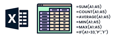
Top Excel Formulas That You Should Know

Microsoft Excel is a valuable spreadsheet software program that can help with many data entry and analytics tasks, and provides a wide range of advanced formulas for calculations and predictions. Excel’s capabilities extend further to visualization, helping people quickly make sense of data for informed decision-making. You can use Excel for data management, including analyzing patterns and relationships between variables. And It can also help you create reports and automate repetitive tasks. Leveling up your Excel skills can boost your productivity and add value to your portfolio, and opening doors to new career opportunities. Get started with these skills Excel users need to know.

What is Excel Formulas?

In Microsoft Excel, a formula is an expression that operates on values in a range of cells. These formulas return a result, even when it is an error. So Excel formulas enable you to perform calculations such as addition, subtraction, multiplication, and division. In addition to these, you can find out averages and calculate percentages in excel for a range of cells, manipulate date and time values, and do a lot more.

Excel Formulas and Functions

There are plenty of Excel formulas and functions depending on what kind of operation you want to perform on the dataset. We will look into the formulas and functions on mathematical operations, character-text functions, data and time, sumif-countif, and few lookup functions.

Let’s now look at the top Excel formulas you must know. In this article, we have categorized Excel formulas based on their operations. Let’s start with the first Excel formula on our list.

1. SUM

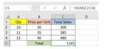
The SUM() function, as the name suggests, gives the total of the selected range of cell values. It performs the mathematical operation which is addition. As you can see above, to find the total amount of sales for every unit, we had to simply type in the function “=SUM(C2:C4)”. This automatically adds up 300, 385, and 480. The result is stored in C5.

2. AVERAGE

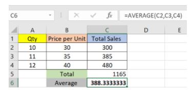
The AVERAGE() function focuses on calculating the average of the selected range of cell values. As seen from the below example, to find the avg of the total sales, you have to simply type in: It automatically calculates the average, and you can store the result in your desired location.

3. COUNT

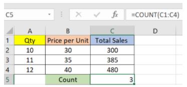
The function COUNT() counts the total number of cells in a range that contains a number. It does not include the cell, which is blank, and the ones that hold data in any other format apart from numeric.

4. POWER

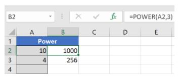
The function “Power()” returns the result of a number raised to a certain power. As you can see above, to find the power of 10 stored in A2 raised to 3, we have to type.

5. CEILING

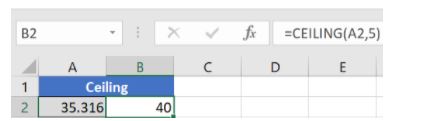
Next, we have the ceiling function. The CEILING() function rounds a number up to its nearest multiple of significance. The nearest highest multiple of 5 for 35.316 is 40.

6.FLOOR

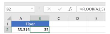
Contrary to the Ceiling function, the floor function rounds a number down to the nearest multiple of significance.The nearest lowest multiple of 5 for 35.316 is 35.

7. LEN

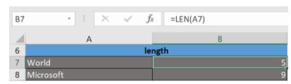
The function LEN() returns the total number of characters in a string. So, it will count the overall characters, including spaces and special characters. Given below is an example of the Len function.

8. NOW()

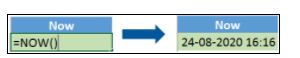
The NOW() function in Excel gives the current system date and time.The result of the NOW() function will change based on your system date and time.

9. TODAY()

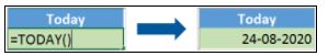
The TODAY() function in Excel provides the current system date.

10.TIME()

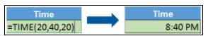
The TIME() function converts hours, minutes, seconds given as numbers to an Excel serial number, formatted with a time format.

11.DATEDIF

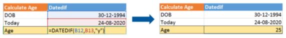
The DATEDIF() function provides the difference between two dates in terms of years, months, or days .In DATEDIF function where we calculate the current age of a person based on two given dates, the date of birth and today’s date

Now, let’s skin through a few critical advanced functions in Excel that are popularly used to analyze data and create reports.

12.VLOOKUP

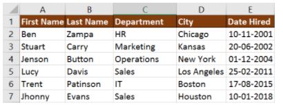
Next up in this article is the VLOOKUP() function. This stands for the vertical lookup that is responsible for looking for a particular value in the leftmost column of a table. It then returns a value in the same row from a column you specify .We will use the below table to learn how the VLOOKUP function works.

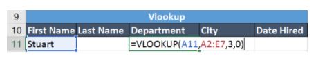
If you wanted to find the department to which Stuart belongs, you could use the VLOOKUP function as shown below:

Here, A11 cell has the lookup value, A2: E7 is the table array, 3 is the column index number with information about departments, and 0 is the range lookup.

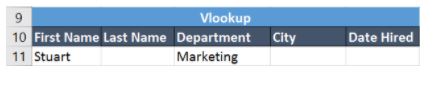
If you hit enter, it will return “Marketing”, indicating that Stuart is from the marketing department.

13. HLOOKUP

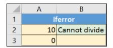
Similar to VLOOKUP, we have another function called HLOOKUP() or horizontal lookup. The function HLOOKUP looks for a value in the top row of a table or array of benefits. It gives the value in the same column from a row you specify.

Below are the arguments for the HLOOKUP function:

Given the below table, let’s see how you can find the city of Jenson using HLOOKUP.

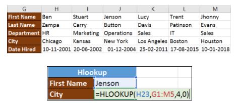
Here, H23 has the lookup value, i.e., Jenson, G1:M5 is the table array, 4 is the row index number, 0 is for an approximate match.

Once you hit enter, it will return “New York”.

14.IF Formula

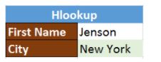
The IF() function checks a given condition and returns a particular value if it is TRUE. It will return another value if the condition is FALSE.

In the below example, we want to check if the value in cell A2 is greater than 5. If it’s greater than 5, the function will return “Yes 4 is greater”, else it will return “No”.

In this case, it will return ‘No’ since 4 is not greater than 5.

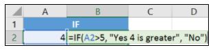
‘IFERROR’ is another function that is popularly used. This function returns a value if an expression evaluates to an error, or else it will return the value of the expression.

Suppose you want to divide 10 by 0. This is an invalid expression, as you can’t divide a number by zero. It will result in an error.

15. LEFT, MID, and RIGHT

Let’s say you have a line of text within a cell that you want to break down into a few different segments. Rather than manually retyping each piece of the code into its respective column, users can leverage a series of string functions to deconstruct the sequence as needed: LEFT, MID, or RIGHT.

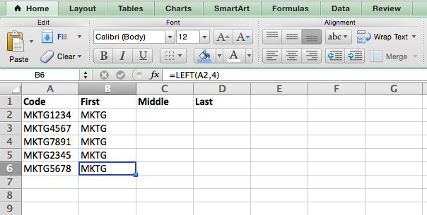
LEFT In Excel Formulas

1. e string
2. Used to extract the first X numbers or characters in a cell.
3. The formula: =LEFT(text, number_of_characters)
  1. Th
4. that you wish to extract from.
5. The number of characters that you wish to extract starting from the left-most character.

In the example below, we entered =LEFT(A2,4) into cell B2, and copied it into B3:B6. That allowed us to extract the first 4 characters of the code.

MID In Excel Formulas

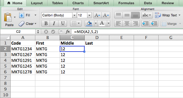
Purpose: Used to extract characters or numbers in the middle based on position.
The formula: =MID(text, start_position, number_of_characters)
Text: The string that you wish to extract from.
Start_position: The position in the string that you want to begin extracting from. For example, the first position in the string is 1.
Number of characters: The number of characters that you wish to extract. In this example, we entered =MID(A2,5,2) into cell B2, and copied it into B3:B6. That allowed us to extract the two numbers starting in the fifth position of the code.

RIGHT in Excel Formulas

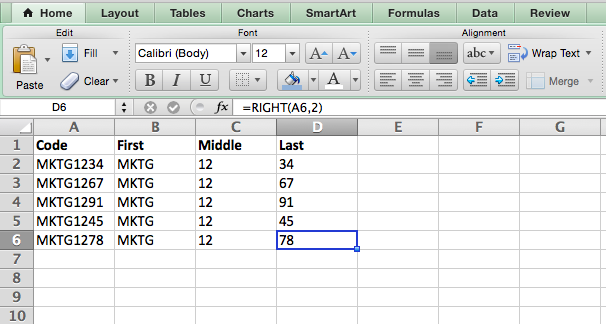
Purpose: Used to extract the last X numbers or characters in a cell.
The formula: =RIGHT(text, number_of_characters)
Text: The string that you wish to extract from.
Number_of_characters: The number of characters that you want to extract starting from the right-most character.

For the sake of this example, we entered =RIGHT(A2,2) into cell B2, and copied it into B3:B6. That allowed us to extract the last two numbers of the code.

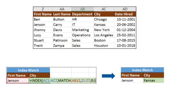
16. INDEX-MATCH

The INDEX-MATCH function is used to return a value in a column to the left. With VLOOKUP, you’re stuck returning an appraisal from a column to the right. Another reason to use index-match instead of VLOOKUP is that VLOOKUP needs more processing power from Excel. This is because it needs to evaluate the entire table array which you’ve selected. With INDEX-MATCH, Excel only has to consider the lookup column and the return column.

17.COUNTIF

The function COUNTIF() is used to count the total number of cells within a range that meet the given condition. Below is a coronavirus sample dataset with information regarding the coronavirus cases and deaths in each country and region. Let’s find the number of times Afghanistan is present in the table.

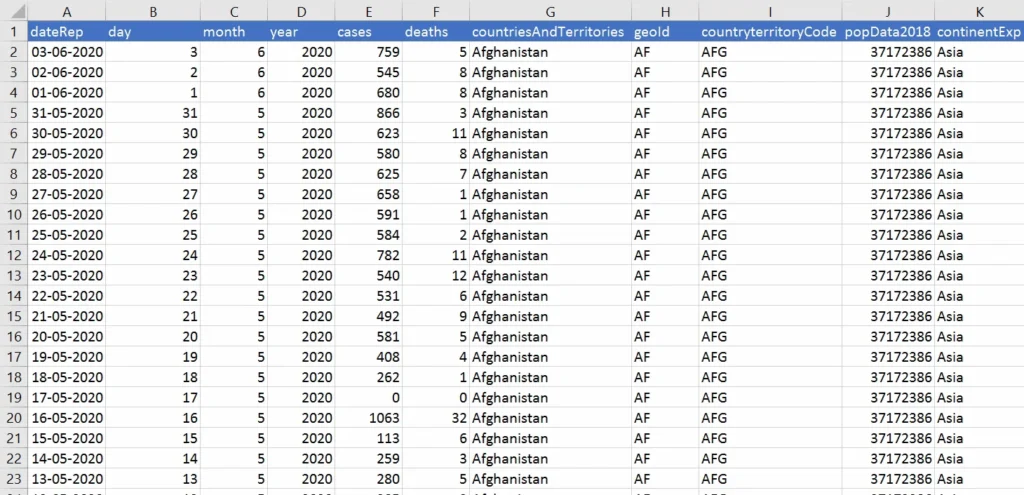
Fig: Countif function in Excel

The COUNTIFS function counts the number of cells specified by a given set of conditions.

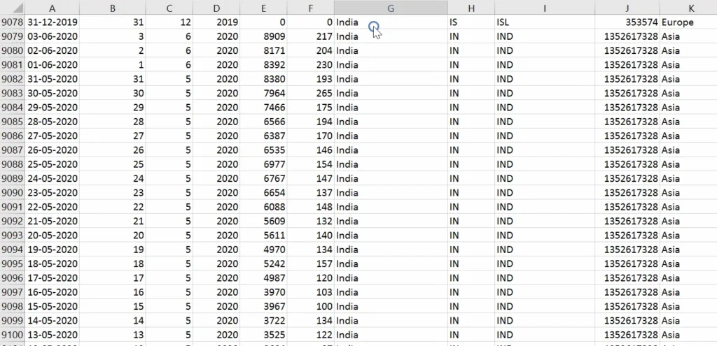
If you want to count the number of days in which the cases in India have been greater than 100. Here is how you can use the COUNTIFS function.

18.SUMIF in Excel Formulas

The SUMIF() function adds the cells specified by a given condition or criteria.

Below is the coronavirus dataset using which we will find the total number of cases in India till 3rd Jun 2020. (Our dataset has information from 31st Dec 2020 to 3rd Jun 2020).

The SUMIFS() function adds the cells specified by a given set of conditions or criteria.

Let’s find the total cases in France on those days when the deaths have been less than 100.

19. Goal Seek in Excel Formulas

Goal Seek is a function in-built in Advanced Excel Functions that allows you to get the desired output by changing the assumptions. The process is dependent on the trial and error method to achieve the desired result.

Let’s look at an example to understand it better.

Example

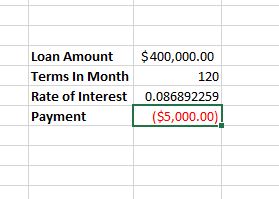
In this example, we aim to find what will be the rate of interest if the person wants to pay

$5000 per month to settle the loan amount.

PMT function is used when you want to calculate the monthly payment you need to pay to settle the loan amount.

Let’s go through this problem in steps to see how we can calculate the interest rate that will settle a loan of $400,000 by $5,000 a month payment.

PMT formula should now be entered in the cell that is the Payment cell adjacent. Currently, there is no value in the rate of interest cell, Excel gives us the payment of $3,333.33 because it assumes the rate of interest to be 0%. Ignore it.

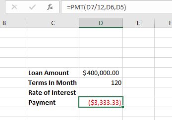
PMT formula should now be entered in the cell that is the Payment cell adjacent. Currently, there is no value in the rate of interest cell, Excel gives us the payment of $3,333.33 because it assumes the rate of interest to be 0%. Ignore it.

Set the monthly payment to -5,000. The deduction in amount signifies the negative value. Set rate of interest as the changing cell.

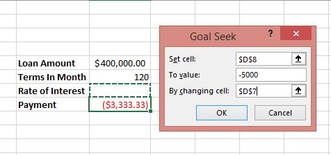
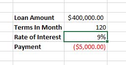
Click OK. You will see the goal seek function automatically gives the interest rate that is required to pay the loan amount.

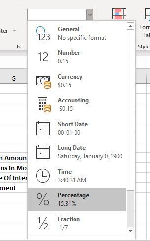
Go to Home > Number and change the value to Percentage.

Your outcome will look like below:

20.What-If Analysis with Solver in Excel Formulas

The method of changing the values to try out different scenarios for formulas in Advanced excel.

Several different sets of values can be used in one or multiple of these Advanced excel formulas to explore the different results.

A solver is ideal for what-if analysis. It is an add-in program in Microsoft Excel and is helpful on many levels. The feature can be used to identify an optimal value for a formula in the cell known as the objective cell. Some constraints or limits are however applicable on other formula cell values on a worksheet.

Solver works with decision variables which are a group of cells used in computing the formulas in the objective and constraint cells. The solver adjusts the value of decision variable cells to work on the limits on constraint cells. This process aids in determining the desired result for the objective cell.

Activating Solver Add-in

On the File tab, click Options.
Go to Add-ins, select Solver Add-in, and click on the Go button.

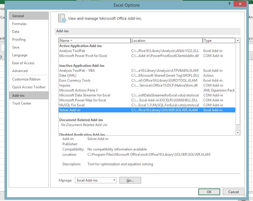
Check Solver Add-in and click OK.

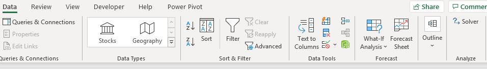
In the Data tab, in the Analyze group, you can see the Solver option is added.

How to Use Solver in Excel

In this example, we will try to find the solution for a simple optimization problem.

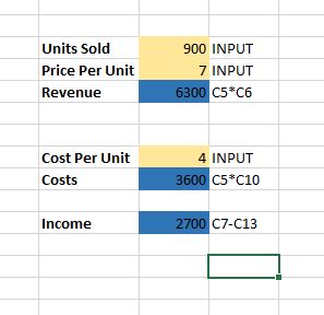
Problem: Suppose you are the business owner and you want your income to be $8000.

Goal: Calculate the units to be sold and price per unit to achieve the target.

For example, we have created the following model:

On the Data tab, in the Analysis group, click the Solver button.
In the set objective, select the income cell and set its value to $8000.
To Change the variable cell, select the C5, C6, and C10 cells.

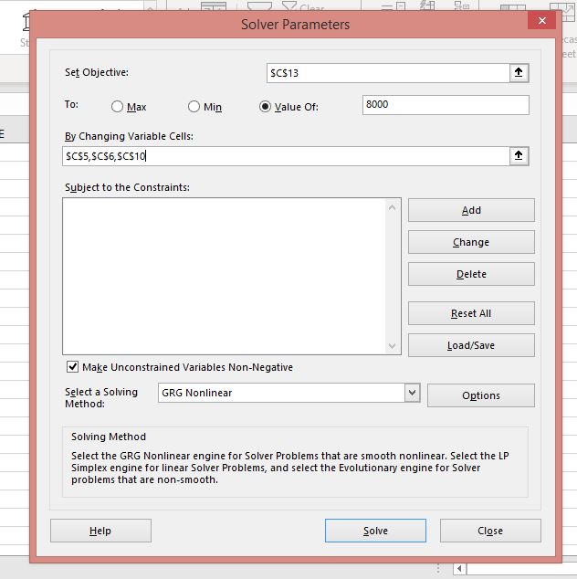
Click Solve.

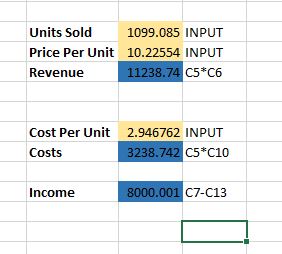
Your data model will change according to the conditions.

Conclusion for Excel Formulas

Excel is a really powerful spreadsheet application for data analysis and reporting. After reading this article, you would have learned the important Excel formulas and functions that will help you perform your tasks better and faster. We looked at numeric, text, data-time, and advanced Excel formulas and functions. Needless to say, Excel knowledge goes a long way in shaping many careers.

Click Below To Avail :